

Introduction: We Simulate the Light. What About the Glass?
Rendering engines have become remarkably good at simulating light. We trace rays, evaluate elaborate material models, and reconstruct indirect illumination, spending large amounts of GPU time approximating how light behaves.
Then we reach the camera.
For most real-time renderers, the camera is a projection matrix with post-processing attached. Depth of field is reconstructed from a depth buffer, chromatic aberration shifts color channels, distortion is a screen-space warp, and vignetting darkens the corners. Each approximation can look convincing on its own.
Real lenses are less cooperative. Their behavior comes from refracting surfaces, aperture geometry, optical materials, and mechanical obstructions. Focusing can change magnification. Stopping down changes the shape of the pupil. Off-axis rays see different aberrations, and different wavelengths do not converge at the same place.
These effects share one physical origin, and simulating them independently creates inconsistencies: circular bokeh over a stretched image, RGB shifts that ignore per-wavelength focus, a vignette that disagrees with the pupil that produced it. For Helio, Pulsar's rendering engine, we wanted those relationships to live in the camera model itself.
Pulsar’s lens subsystem combines real-time optical approximations with prescription-derived data. Both use the same reconstruction pipeline, so effects from modeled lenses and authored optics can work together.
The following sections explain how the optical model reaches Helio’s WGSL compute pipeline and how the Rust camera component supplies its settings.
The code discussed comes from Helio's camera lens component and WGSL lens shader. The sections on literal surface-by-surface tracing describe the physical model and reference algorithms, not code from the prescription generator, which is not included here.
Drag the slider to compare the same scene without and with the lens simulation enabled.
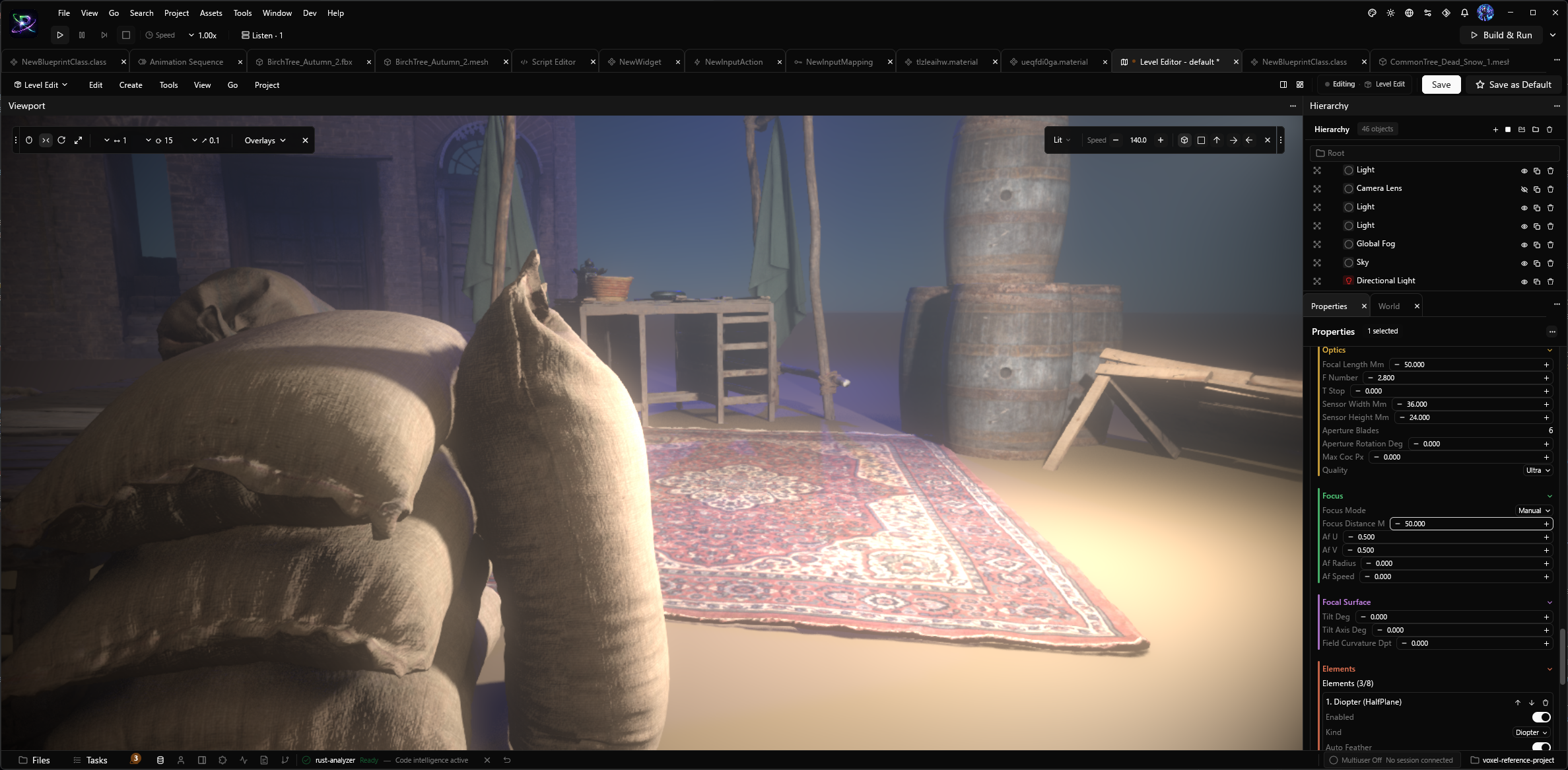
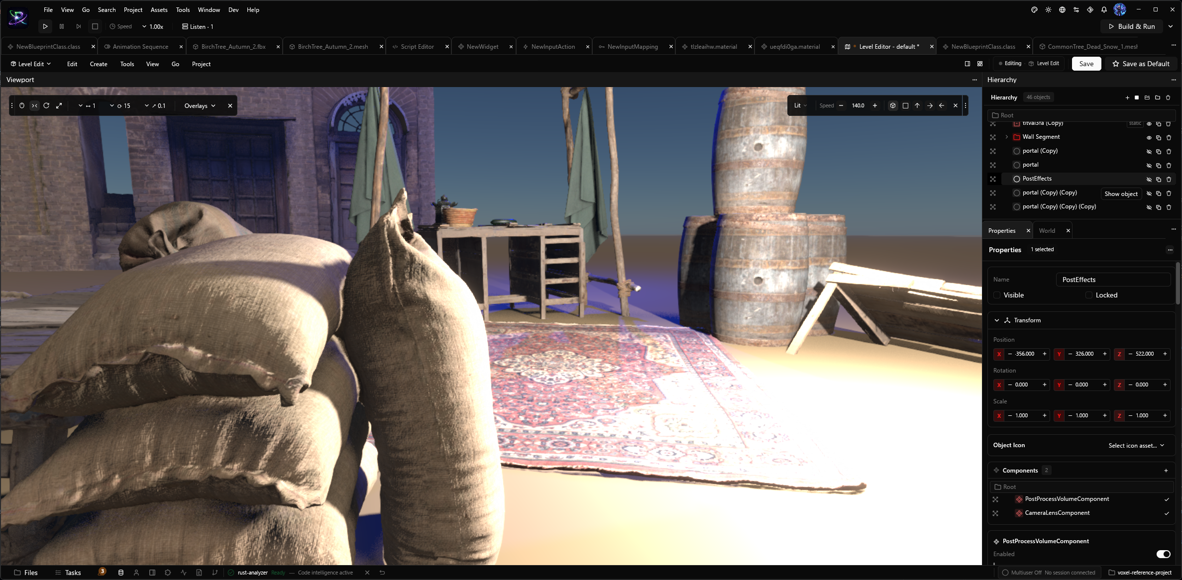 Without lens simulationWith lens simulation
1. Representing a Lens as an Optical System
A pinhole camera maps each sensor position to one scene direction. A real lens has a finite aperture, so light reaching one sensor position can travel through many parts of the pupil and across many wavelengths. A literal simulation would trace and shade all those paths for every pixel, every frame—too expensive for this real-time pipeline.
Helio instead represents the lens with four related quantities:
- Ray map: where each sensor position samples the scene, including projection, distortion, and wavelength-dependent shifts.
- Focus field: the scene distance that should appear sharp at each sensor position.
- Pupil: which paths through the aperture contribute and how strongly, shaping defocused highlights.
- Transmission: how much light survives, including vignetting and filters.
These values can be authored directly or baked from a physical lens prescription, then evaluated against the scene's existing color and depth buffers. This shared representation keeps related effects connected: distortion changes where the image is sampled, focus sets blur, the pupil shapes it, and transmission controls brightness.
1.1 Optical operations are order-dependent
Blurring then distorting does not produce the same result as distorting then blurring. A nonlinear ray map changes local magnification, so a circular blur can become stretched or rescaled. Helio computes defocus in the undistorted scene, adjusts it for local magnification, and applies the ray map during final composition. This makes distortion part of the optical reconstruction rather than a separate screen-space effect.
2. The Camera Lens Component
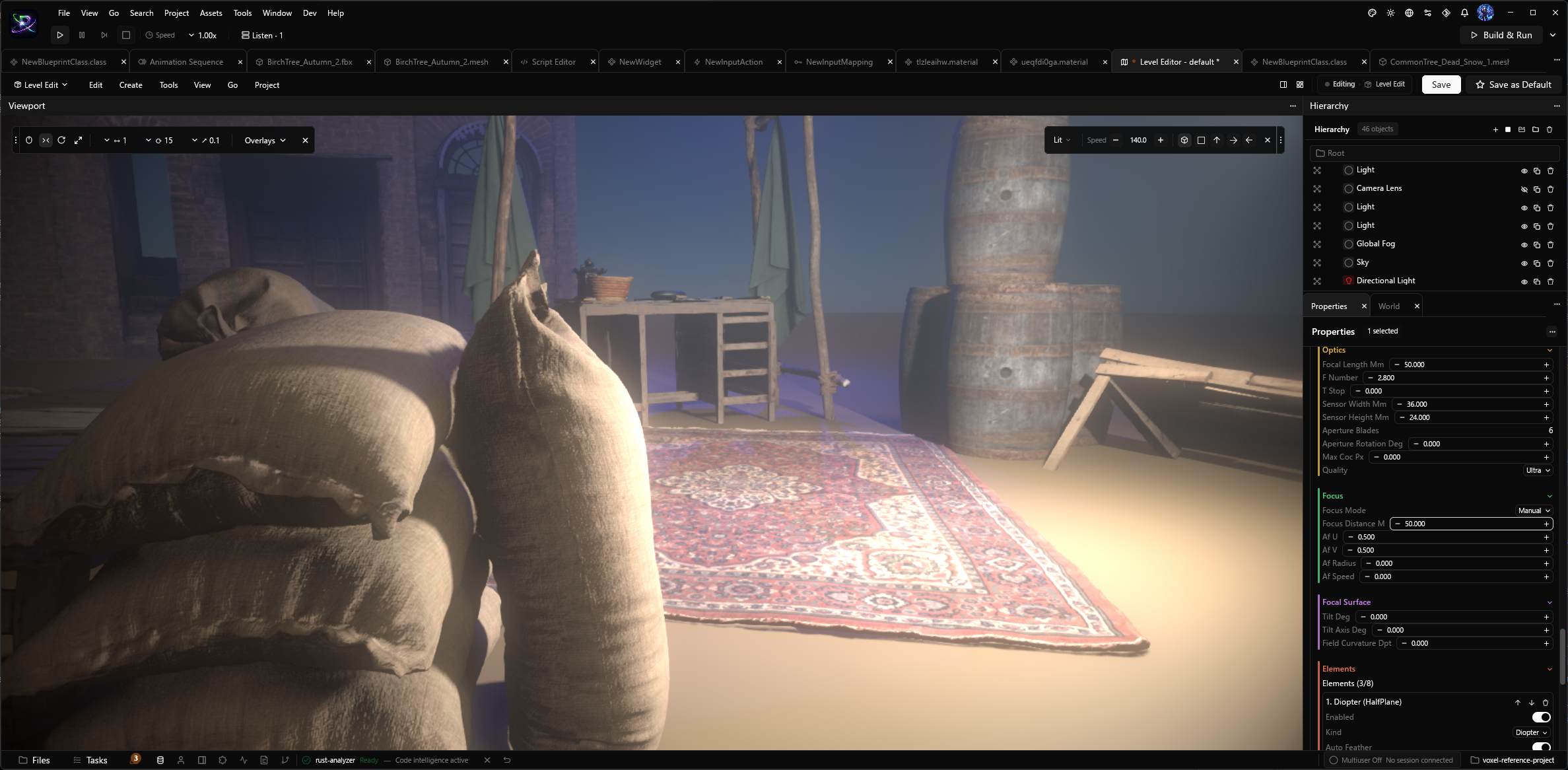
The editor-facing CameraLensComponent belongs to a camera and holds its optical settings, focus controls, quality level, and ordered element stack. Its serializable, reflected fields are editable in the inspector; Helio converts them through SceneDB into packed GPU rows.
2.1 View selection
The lens pass selects the first enabled lens row matching the active view_id (the editor viewport uses view zero). This lets editor, runtime, and secondary cameras use different optics. Hiding the owning object does not disable its lens.
2.2 GPU buffers and packed rows
The component writes source rows to camera_lens_sources and packed element rows to lens_elements; the environment join publishes eligible sources as camera_lenses for the render pass. Elements occupy contiguous blocks—eight slots per authored lens, with a shader ceiling of 32—so the shader can address them by start index and count instead of following sparse entity indices. Removing a lens frees and zeroes its allocation.
CameraLensSourceRow is a 96-byte #[repr(C)] array of words. A compile-time assertion checks its size against the rendering pass's LensComponent, and conversion uses a byte-preserving bytemuck read. The layout is an internal Rust/WGSL contract: changes to field order, size, or alignment must stay coordinated.
3. The Thin-Lens Equation and Circle of Confusion
A lens focused at one distance brings objects at that distance to a point on the sensor. Objects closer or farther away form a small blur disk called the circle of confusion (CoC). Its size grows with aperture and distance from the focus plane.
For focal length , f-number , object distance , focus distance , sensor width , and image width , the approximate blur diameter in pixels is:
This equation gives the blur magnitude; all distances must use consistent units. Helio also keeps the blur sign: foreground blur is negative and background blur positive. That distinction lets reconstruction keep near and far contributions separate, since foreground blur can cover background detail.
3.1 A practical example
Converting the 50 mm focal length to 0.05 m, a lens at f/1.4 focused at 3 m produces about a 25.8-pixel CoC for a point 5 m away on a 3840-pixel-wide image using a 36 mm sensor. Stopping down halves that blur at f/2.8 and halves it again at f/5.6.
Large blur disks are costly to reconstruct, so Helio clamps them to the authored max_coc_px. This is a rendering limit, not a physical property: the real lens may produce a larger blur than the real-time pipeline attempts to reproduce.
3.2 F-number and T-stop
The f-number describes aperture geometry; the T-stop describes how much light passes through the lens. Transmission loss makes the T-stop numerically larger than the f-number, but it does not change the geometric blur size. Helio exposes both so brightness and depth of field remain separate controls.
4. Focus Is a Surface, Not Necessarily a Distance
A thin-lens model assumes one focus distance across the frame. Tilt-shift optics, field curvature, and split diopters break that assumption: different sensor regions can focus at different distances. Helio represents focus as a spatial field. It often stores focus in diopters—the inverse of distance in meters (), so infinity is zero and optical powers combine naturally.
4.1 Tilted focal plane
Tilting the focal plane changes which scene distance appears sharp across the image. Helio evaluates a geometric tilted-plane model from the camera projection and bounds rays that approach parallel to the plane, where the calculated distance would diverge. This captures the primary depth-of-field effect without physically moving lens groups; real tilt mechanisms can also change magnification, aberrations, and pupil shape.
4.2 Field curvature
Some lenses focus a flat object onto a curved image surface. Helio models the focus power as , where is distance from the image center. For example, a camera focused at 5 m with a +0.1-diopter corner correction focuses the corner near 3.3 m, so a 5 m subject can be sharp in the center and soft at the edge. The effect is most visible at large apertures.
4.3 Split diopters
A split diopter changes focus over only part of the image. Its optical power is derived from the difference between the target region's focus and the camera's current focus. Near the boundary, rays may pass through both the diopter and the uncovered lens, producing overlapping blur patterns rather than one intermediate focus.
Helio preserves two focus distances and a seam weight for reconstruction. The component also exposes seam darkening and mount distance; stopping down narrows the visible transition because the transmitted ray bundle is smaller.
4.4 Sweet spots
A sweet-spot lens keeps one image region relatively sharp and adds blur outside it. Helio models this as a region-specific element that can combine with field curvature and pupil shaping.
Split focus can use a half-plane, angled seam, ellipses, radial band, or polygon. The captures use the same scene with a fast 85 mm lens so the focus regions are easier to see.
5. The Pupil Function and Why Bokeh Has Shape
The CoC says how large an out-of-focus point becomes; the pupil determines what that blur looks like. A circular aperture gives round highlights, iris blades make polygonal ones, and off-axis barrel clipping can create cat's-eye shapes. Anamorphic optics can stretch the pupil.
Helio separates the pupil’s shape from its intensity profile; their product determines the weight of each sampled path through the aperture. The shader supports curved iris blades, field-dependent barrel clipping, central obstruction, spherical-aberration profiles, onion-ring modulation, and apodization. These change the distribution of blur without automatically changing total brightness; transmission loss is handled separately.
Prescription-derived pupil masks can replace the analytic shape with traced coverage. Helio estimates pupil area and near/far profile means using 96 samples, then normalizes the reconstruction so changing bokeh shape does not arbitrarily brighten or darken a source.
The anamorphic examples show how pupil stretch changes highlight shape. The next set changes the pupil's intensity profile, softening its center or emphasizing rings and edges.
6. Spectral Optics and Chromatic Aberration
Glass bends different wavelengths by different amounts. This dispersion creates two distinct effects: longitudinal chromatic aberration shifts the focus distance, while lateral chromatic aberration shifts image position or magnification. Helio keeps them separate: focus changes affect CoC, while lateral shifts affect the ray map.
The supplied shader samples roughly 400–700 nm. Quality settings use 3, 7, or 16 wavelength samples, accumulated with channel weights into an RGB result. This is a spectral approximation over an RGB scene image, not a full spectral renderer; RGB values cannot uniquely recover the original light spectrum.
A physical lens tracer evaluates each material's wavelength-dependent refractive index at every surface. Optical designs can combine glasses to reduce color error, though residual shifts may remain. In Helio, wavelength-dependent focus can give red, green, and blue different blur sizes, while wavelength-dependent ray maps can shift their positions. At a split-diopter seam, two focus configurations may be evaluated per channel, for up to six gather lanes.
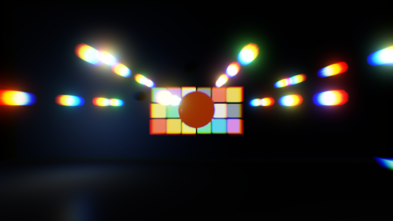
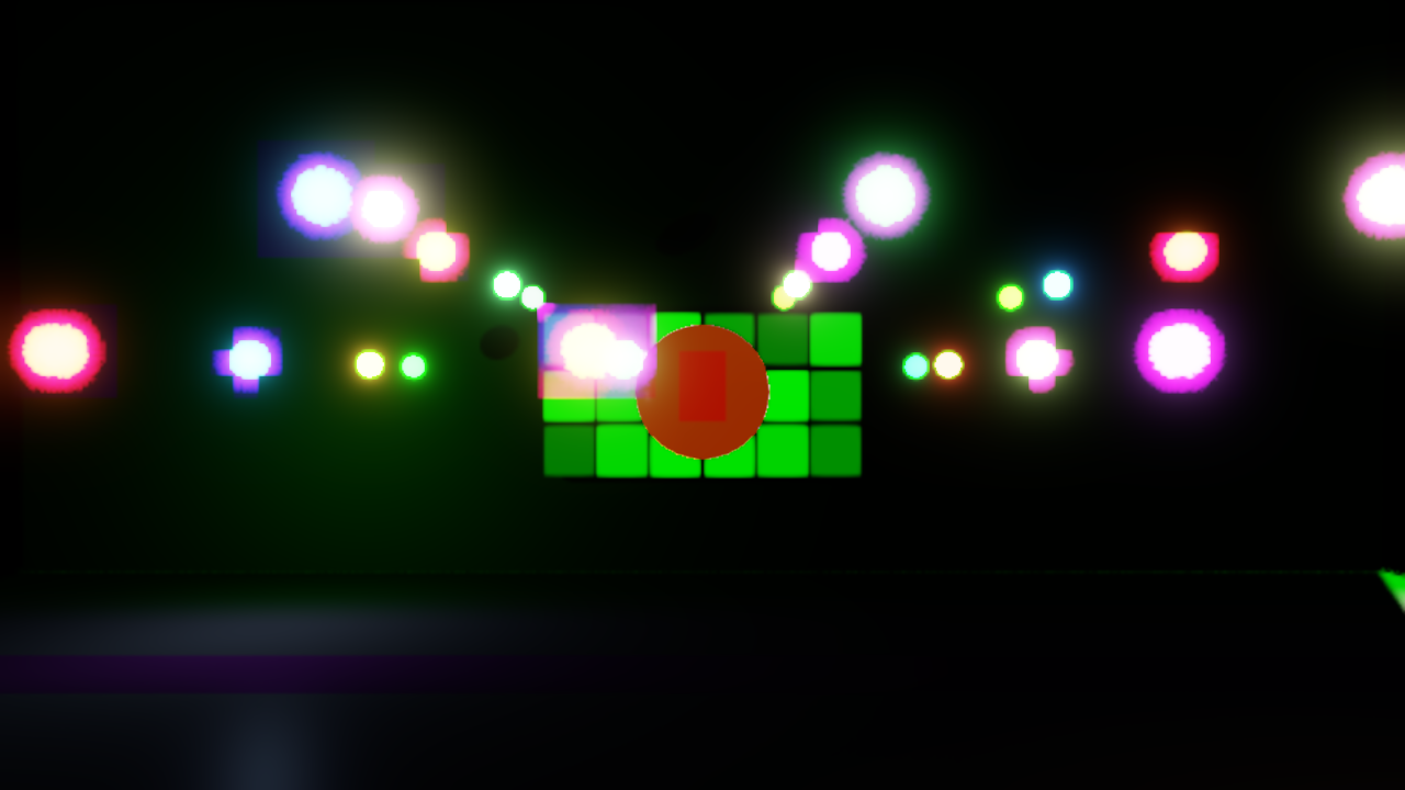 Longitudinal chromatic aberrationLateral chromatic aberration
7. Geometric Ray Mapping
The ray map converts sensor coordinates into scene sampling coordinates. Elements are applied in order: anamorphic squeeze followed by radial distortion generally differs from the reverse order, so Helio preserves the authored stack.
Helio supports rectilinear, equidistant, equisolid-angle, orthographic, stereographic, cylindrical, Panini, and Kannala–Brandt projections. They trade off different geometric properties: for example, rectilinear keeps ordinary perspective lines but expands dramatically near 90 degrees, while equidistant makes image radius proportional to ray angle.
The system also supports Brown–Conrady radial and tangential distortion, lens shift, and anamorphic mappings. A calibration model may describe a forward mapping while a render pass needs the inverse; that can require an iterative solve or fitted approximation.
Nonlinear maps change local image magnification, which also changes blur size. Helio uses the map's Jacobian determinant as a scalar area-scale correction for the CoC. This is cheaper than transforming every blur into an anisotropic ellipse, but it does not capture all local rotation, shear, or directional stretching.
The paired examples below isolate two common radial-distortion directions; use the gallery above to compare the wider range of mappings and projections.
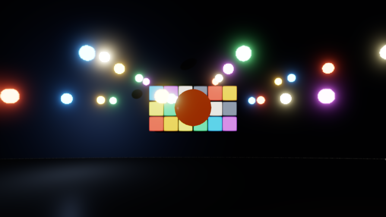
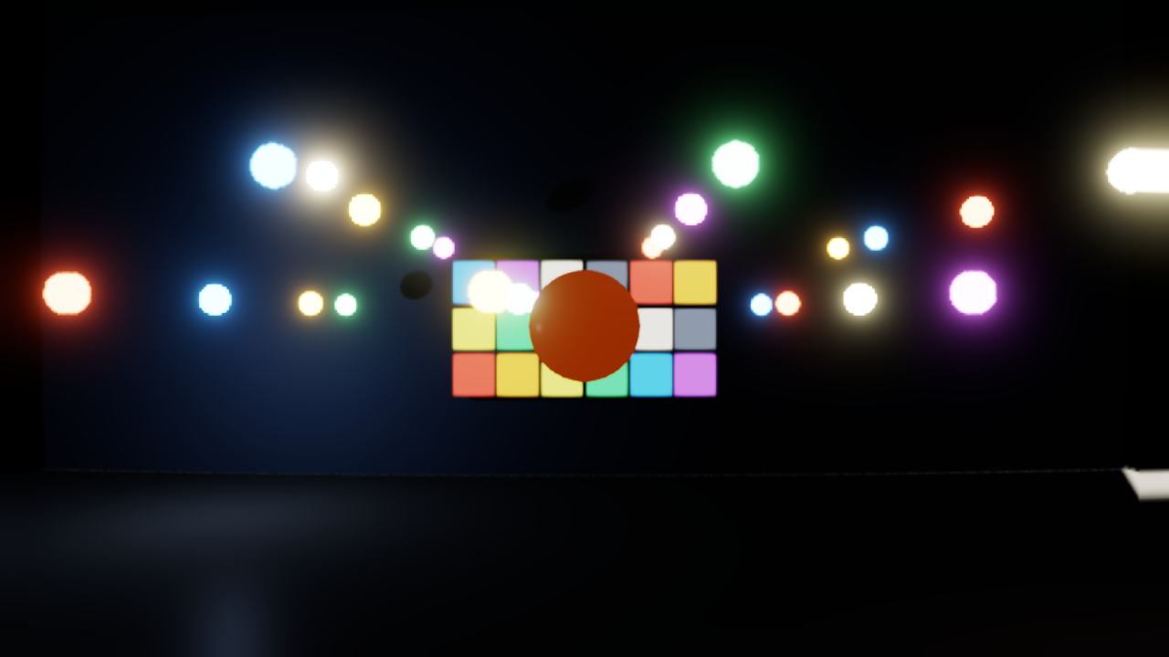 Barrel distortionPincushion distortion
8. The Compute Pipeline
The lens pass runs as a sequence of WGSL compute stages:
| Stage | Work |
|---|---|
cs_resolve | Select the active lens, resolve focus and overscan, set indirect dispatches |
cs_coc | Compute signed blur and focus-field metadata |
cs_tiles / cs_dilate | Bound blur footprints and the gather search region |
cs_prefilter | Separate near and far samples at half resolution |
cs_gather | Reconstruct blur using source CoC and pupil weights |
cs_composite | Combine sharp, near, and far layers with mapping and transmission |
| Optional aberration stages | Apply point-spread effects, diffusion, halation, and contaminants |
When no lens is enabled, resolve suppresses unnecessary stages and the composite pass copies the source. This allows per-view lens activation without rebuilding the pipeline.
The CoC pass writes one rgba16float texture. Its channels hold primary and secondary signed CoC, split-focus seam blending, and focus-field transmission. Keeping them together supports ordinary depth of field and split-diopter reconstruction.
Tile analysis summarizes CoC values in each 16×16 region. Dilation expands those bounds because blur sources can lie outside the destination tile. Before gathering, a 2×2 full-resolution footprint is classified as near or far; preserving those classes avoids mixing foreground and background colors across silhouettes before depth-aware reconstruction. This reduces a common artifact but cannot recover hidden geometry.
9. Scatter-as-Gather
A defocused source contributes light over an area of the image. A direct scatter pass would write each source into many destination pixels, creating parallel write conflicts. Helio instead starts at each destination and gathers nearby sources, but weights each source using its own blur radius and pupil. This is closer to the optical behavior than applying one destination-centered blur kernel.
A simplified reconstruction is a weighted average:
Here is the source blur radius. The pupil decides whether a destination lies inside that source's blur footprint; the inverse-square term spreads its energy over the larger area.
The shader samples the neighborhood on a golden-angle spiral, rotating the pattern per pixel to reduce visible alignment. Small blur disks use fewer taps; quality settings cap the gather at 24 or 56 taps.
Near and far contributions use separate accumulators. The near layer includes coverage and composites over the far layer, because foreground blur can cover background detail while background blur cannot cover an opaque foreground object. The reconstruction still uses visible color and depth only; section 17 discusses the hidden-geometry limit.
10. Physical Lens Prescriptions
Analytical functions are fast and easy to art-direct. A physical prescription describes the lens's ordered surfaces, spacing, materials, and apertures, letting optical behavior be derived from a modeled design instead.
The component includes thin-lens, Cooke-triplet, and double-Gauss choices. Their traced behavior is packed into a GPU prescription bank; the runtime shader reads lookup data rather than tracing every surface for every pixel.
10.1 What the prescription supplies
The bank stores wavelength-dependent ray mapping, relative illumination, pupil coverage, field curvature, and point-spread analysis. Runtime helpers expose these as rx_tan, rx_vignette, rx_mask, and rx_analysis. The shader interpolates between sampled field and wavelength values, producing a continuous approximation to the traced lens.
The pupil mask can represent irregular off-axis coverage from internal surfaces and mechanical obstructions. Relative illumination varies by field position and aperture; the bank samples f-number on a logarithmic scale. This captures lens-specific falloff more directly than a generic cosine-fourth-power estimate.
10.2 Point-spread analysis
Prescription analysis provides field curvature, radial and tangential spot widths, and a signed coma-tail share and length. These compact values capture several geometric aberrations without storing an arbitrary two-dimensional diffraction pattern. When prescription-derived PSF data is active, Helio avoids applying the corresponding authored coma, astigmatism, or corner-softness effects a second time.
11. Literal Multi-Surface Ray Tracing
Prescription data comes from tracing rays through a sequence of curved optical surfaces. At each surface, an offline tracer finds the ray intersection, checks the clear aperture, and bends the ray according to the wavelength-dependent refractive indices on either side. Aspheric surfaces require a numerical intersection solve; the tracer must also handle surface order, medium changes, numerical tolerances, and total internal reflection.
A tracer can sample wavelength, field position, aperture, focus, and pupil position, then record ray direction, illumination, pupil coverage, field curvature, and spot behavior. Even a modest sample grid produces millions of rays and tens of millions of surface interactions, so this is an offline or asynchronous bake. The real-time pipeline compresses the result into lookup functions rather than tracing every pixel each frame.
The supplied files establish the prescription-consuming path, not the offline generator.
12. Practical Details
Overscan
Strong distortion, fisheye, lens shift, and some anamorphic mappings can ask for scene samples outside the rendered frame. Clamping stretches edge pixels; leaving them black creates borders. Helio renders a wider field and maps it back to the nominal frame.
camera_lens_view_overscan estimates the needed coverage from 64 frame-boundary samples and caps the optical request at 16; the host camera applies at most 2. At constant pixel density, rendered area grows with the square of the overscan factor: 1.25× coverage costs about 56% more pixels, while 2× costs four times as many. The actual cost depends on whether the host increases resolution, field of view, or both.
Depth and optical distance
Defocus needs distance in scene units, while the depth buffer stores projected depth. Helio reconstructs view-space distance through its shared reversed-Z depth utilities; the exact conversion depends on the camera projection.
With upscaling, depth and color may have different resolutions. The lens shader samples a 2×2 depth footprint and chooses the nearest value, favoring foreground edges so they are not assigned background focus distances. This helps silhouettes but cannot recreate missing depth layers. Sky pixels use a large finite distance (SKY_DISTANCE 1.0e5, MAX_DISTANCE 1.0e6) so infinity does not propagate through the CoC calculation.
Autofocus
Autofocus samples a region around the authored focus point instead of relying on one depth pixel. It averages inverse distances (diopters), which gives nearby objects more influence: equal samples at 1 m and 9 m produce a target near 1.8 m, rather than the 5 m midpoint. A small foreground obstruction can therefore pull focus unexpectedly.
Focus state persists between frames in diopters, and af_speed controls the adjustment rate; zero means instant focus. Interpolating in diopters tracks optical power better than interpolating raw distance, especially at close range.
Custom optical elements
The lens system supports custom WGSL hooks. The shader ships default user_ray_map, user_transmission, and user_focus functions with identity behavior, gated by USER_ENABLED, and the host can replace the marked snippet block when constructing the pass. Flags decide whether a user element participates in mapping, transmission, focus, or spectral behavior.
A custom ray map could approximate an unusual prism, a custom focus function could introduce a nonstandard focal surface, and a custom transmission function could represent an experimental filter. The hooks operate within the existing optical representation, so gather and composition still reconstruct the image and custom elements do not need a separate renderer.
Presets and authoring
The lens system exposes named presets for common optical configurations.
The supplied component includes:
| Preset | Primary behavior |
|---|---|
| Standard 50 mm f/2.8 | Conventional prime lens |
| Portrait 85 mm f/1.4 | Large-aperture portrait optics |
| Split Diopter 2-Way | Two focus regions |
| Split Diopter 3-Way | Three-region split-focus configuration |
| Tilt-Shift Miniature | Tilted focal surface |
| Lensbaby Sweet Spot | Localized sharp region |
| Anamorphic 2× | Anamorphic projection and pupil behavior |
| Vintage Helios Swirl | Swirling off-axis bokeh |
| Fisheye 8 mm | Wide-angle nonlinear projection |
| Underwater Flat Port | Refraction through a flat underwater port |
| Pro-Mist Quarter | Diffusion |
| Black Pro-Mist Eighth | Highlight diffusion |
| Rainy Lens | Water-drop effects |
| Star Filter 6pt | Six-point star response |
| Film Halation | Film-like highlight halos |
| Grad ND 3 Stop | Graduated neutral density |
| Double Gauss 50 mm f/2 Traced | Prescription-derived optical behavior |
Presets are data over the same component fields, not separate implementations. The component's resolved() method produces the effective configuration, and bake_preset() copies a preset into editable fields and switches the selection to Custom. A traced double-Gauss, an anamorphic preset, or a split-diopter setup can all serve as a starting point for a more specialized lens.
Numerical stability
Optical calculations become sensitive near the focal length, at projection limits, at infinite focus, and when spectral samples leave the rendered frame. The shader checks for non-finite values and uses a bounded() helper to substitute fallbacks and clamp inputs.
Resolved runtime values are clamped—for example, focal length to 8–600 mm and f-number to 0.7–32. Some editor ranges are broader, so a value may stop changing once it reaches the runtime limit. Rectilinear projection is capped near 85 degrees because its image radius diverges toward 90 degrees. Half-precision intermediate textures save bandwidth but can quantize or saturate; the shader bounds radiance and protects normalization denominators to avoid catastrophic failures.
13. Aberrations Beyond Depth of Field
A perfect geometric lens forms a point at focus, while real optics produce finite spot sizes and asymmetric point-spread functions. Helio represents prescription-derived spots with radial and tangential Gaussian widths in sensor millimeters, then converts them to pixels using the sensor and image widths. Authored and prescription-derived coma add a directional tail to the point-spread function; astigmatism uses different radial and tangential widths, which can change with field position and focus.
The same image-space aberration path approximates several filter effects:
- Diffusion: Pro-Mist, Black Pro-Mist, Glimmerglass, fog, and spherical glow use multiple image-pyramid scales to create different halo profiles.
- Star filters: Directional streaks use authored point count, rotation, length, intensity, and falloff. This approximates the filter signature rather than simulating diffraction.
- Halation: Strength, radius, tint, and tail controls create film-like halos around highlights.
- Contaminants: Water masks refract through drop regions and normals; smears add directional diffusion; dirt adds localized scattering and transmission loss. These use image-space masks rather than fluid or particle simulation.
14. Localized Optical Elements
Optical effects can apply to selected image regions: half-planes for split diopters, ellipses for sweet spots, directional regions for graduated filters, and masks for irregular water or dirt patterns. Polygon and radial-band regions are also supported. Coordinates are centered on the frame and normalized by image aspect ratio , spanning horizontally and vertically.
Mask regions select a texture-array layer and color channel, with scaling, translation, inversion, and tiling. A transparent fallback prevents a missing host texture from applying an effect across the whole image.
Elements act on shared optical quantities in stack order: ray maps compose coordinates, transmission attenuates, focus changes the focal field, pupils shape blur, and aberrations modify the reconstructed image. Their interactions are resolved by the common pipeline rather than by independent image filters.
This larger gallery is scrollable. It covers vignettes, filters, underwater ports, prisms, and localized mask effects.
15. Performance: Where the GPU Time Goes
The largest cost controls are half-resolution gathering, bounded tap counts, tile-based footprint analysis, indirect dispatch suppression, and precomputed prescription data. At 3840×2160, half-resolution gathering has about 2.1 million pixels; at 56 taps and three active spectral lanes, the rough upper estimate is 348 million candidate evaluations. This is a workload estimate, not a texture-fetch count: pixels often use fewer taps, tests reject samples, and lanes may reuse fetched data.
An rgba16float full-resolution texture is about 63.3 MiB; a half-resolution one is about 15.8 MiB. The actual intermediate-memory cost depends on resource lifetimes and aliasing. Spectral quality uses 3, 7, or 16 samples, though the longitudinal-CA gather uses RGB lanes rather than 16 independent defocus lanes.
Gather accumulators can increase register pressure and reduce occupancy, while irregular sampling can strain memory access. The source establishes the architecture, not measured performance. Useful target-hardware measurements include GPU time per pass, tap distribution, occupancy, cache behavior, spectral-lane use, prescription lookup cost, and overscan cost.
16. Validating the Optical Model
Test optical behavior against measurable outcomes rather than judging by appearance alone. For CoC, render point sources at known distances and compare the measured blur with the relationship in section 3; halving the f-number should roughly double the geometric blur, and near/far classification should change at the focal surface.
- Pupil energy: A uniform image should remain uniform under normalized circular, polygonal, obstructed, apodized, and prescription-derived pupils. Test transmission separately so a neutral-density filter darkens the image without changing kernel shape.
- Distortion: Compare a grid of known world points against the analytical or prescription mapping at center, edges, and corners; report mean, RMS, and maximum error.
- Chromatic aberration: Check channel centroids and magnification for lateral CA, and per-channel focus and blur size for longitudinal CA.
- Prescription comparison: Compare against a converged ray trace across field, aperture, focus, and wavelength, including illumination, pupil coverage, spot shape, and focal-surface displacement.
- Temporal stability: Measure sequences while focus, camera position, depth edges, or jitter change, especially around bright blurred sources and foreground silhouettes.
17. Where Physical Accuracy Still Has Limits
Helio reconstructs lens behavior from an existing scene color and depth image. This is much cheaper than rendering the scene for every pupil sample, but it limits visibility: different parts of a real lens pupil can see different surfaces, while a single color/depth layer cannot reveal background radiance hidden behind a foreground object. Near/far separation reduces common halos but cannot recover arbitrary hidden geometry. A ray-traced or layered solution could improve disocclusion at additional rendering and memory cost.
17.1 Wave optics
Geometric rays do not model diffraction. In wave optics, a pupil's amplitude and phase produce a point-spread function through a Fourier transform:
This relationship explains diffraction spikes, Airy patterns, and wavefront-aberration effects. Helio approximates some related image signatures but the supplied shader does not establish a general wave-optics FFT implementation.
17.2 Coatings, ghosts, and dynamic prescriptions
Coatings vary with wavelength, incidence angle, and polarization; internal reflections can create ghosts and flare. A complete simulator would trace reflected as well as transmitted paths, which Helio's supplied shader does not do.
Focusing or zooming can move lens elements and change focal length, distortion, pupil magnification, field curvature, and aberrations. Helio supports focus breathing as a ray-map element; a fuller model could interpolate between traced optical states, at the cost of larger datasets and careful interpolation.
18. The Architecture Behind the Image
Analytical and prescription-derived lenses share one reconstruction pipeline: the ray map selects scene samples, the focus field sets defocus, the pupil shapes the blur, and transmission controls throughput. Camera-owned settings become SceneDB GPU rows, so optical elements compose without teaching the scene renderer about each one. The result remains an approximation of full ray tracing, but related effects respond to a shared camera model: aperture changes the pupil and blur, focus changes the focal field, and wavelength can affect both mapping and focus.